Benchmarking run time#

When changing ASPECT’s code it can be useful to check if and how much the new changes affect the run time of ASPECT. To test this, one could compile ASPECT in release mode on the main branch and on the branch with the changed code (e.g. feature branch), run both models and time both runs. The problems is that this is not very reliable, because your computer might be doing something in the background on one but not both of the runs.

However, measuring the performance of code is a complex topic that can be approached in many different ways, for example:

Collecting statistics about the different tasks the processor has to execute and measuring their influence on the performance, e.g. using the tool perf as described here: https://integrated-earth.github.io/2023/02/03/perf.html.
Running a virtual machine that is instrumented to count every single instruction that is executed and displays the amount of time spent in each line of code using the tool callgrind.
Executing a program many times with and without the changed code and comparing the run time statistics, e.g. using the tool cbdr. This is the approach discussed on this page.

Note

When running timing benchmarks, always make sure to compile in release mode. Debug mode is for testing model implementations, but the change to release mode affects the performance of different parts of the code differently. Useful timing information can only be generated in release mode (see Debug or optimized mode).

As mentioned above, one option to compare performance is to run both executables after each other in a random order. This is what the program cbdr can do for you. It can also analyze and report the result.

This program can be installed with cargo (see Install Cargo button), with cargo install cbdr. To generate the run data, the program is run with cbdr sample --timeout=900s main:/path/to/build-main/aspect-release /path/to/test.prm features:/path/to/build-feature/aspect-release /path/to/test.prm > results.csv. This command runs both the main and feature branch executable to “warm up” and then it keeps randomly selection one of the two executables and write the timings out to results.csv until the timer reaches 900 seconds.

The results.csv can then be summarized with cbdr analyze <results.csv, which produces the following output:

           main           feature        difference (99.9% CI)
sys_time   0.868 ± 0.071  0.916 ± 0.051  [  +1.5% ..   +9.7%]
user_time  7.216 ± 0.133  7.112 ± 0.100  [  -2.4% ..   -0.5%]
wall_time  6.556 ± 0.045  6.498 ± 0.046  [  -1.3% ..   -0.5%]
samples    66             74

You can ignore the sys_time in the output above. It just shows how much time the programs spends on operating system kernel calls. The user time is how much the program actually spends on your processor and the wall time is how much time the program takes if you measure it by having a stop-watch next to your computer. In this case it is nearly the same, but if you run it with many processors, the user time might be much larger then the wall time.

In this case the feature branch is measured by the wall time between 1.3% and 0.5% faster than the main branch with a 99.9% confidence interval. This means that in this case we can have reasonable confidence that the feature branch is a bit faster than the main branch.

The cbdr program can also create a graphical output in a vega-lite format through the command cbdr plot <results.csv > results.vl. This can then be converted to a png through vl-convert with the command vl-convert vl2png --input results.vl --output results.png.

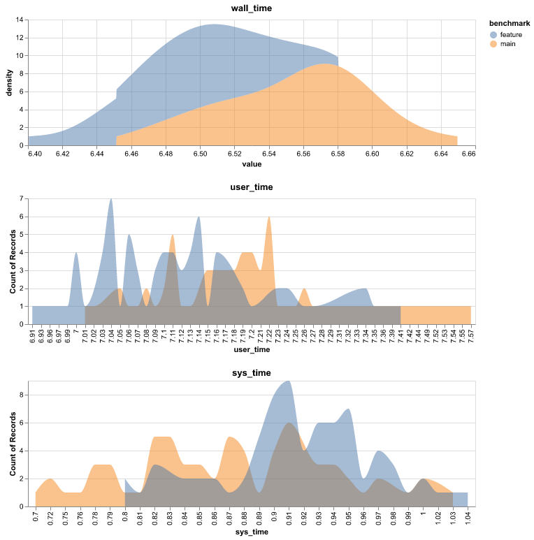
benchmark runtime graph — Fig. 294 Example graph created for the same run as the table above.#